Usage
Using SmartPeak GUI
After successful installation of SmartPeak, on Windows open menu start and browse for relevant icon, you can also find the shortcut on desktop.
If built SmartPeak from the source code, from the build directory run
./bin/SmartPeakGUIfor Mac and Linux, or./bin/[Debug or Release]/SmartPeakGUIfor Windows. Or double-clickSmartPeakGUIexecutable in the file browser of your OS.Start the session with
File | Load session from sequenceChoose the corresponding directory with
Change dir. The path to example folder can be shortened to f.e./data/GCMS_SIM_UnknownsSelect the sequence file
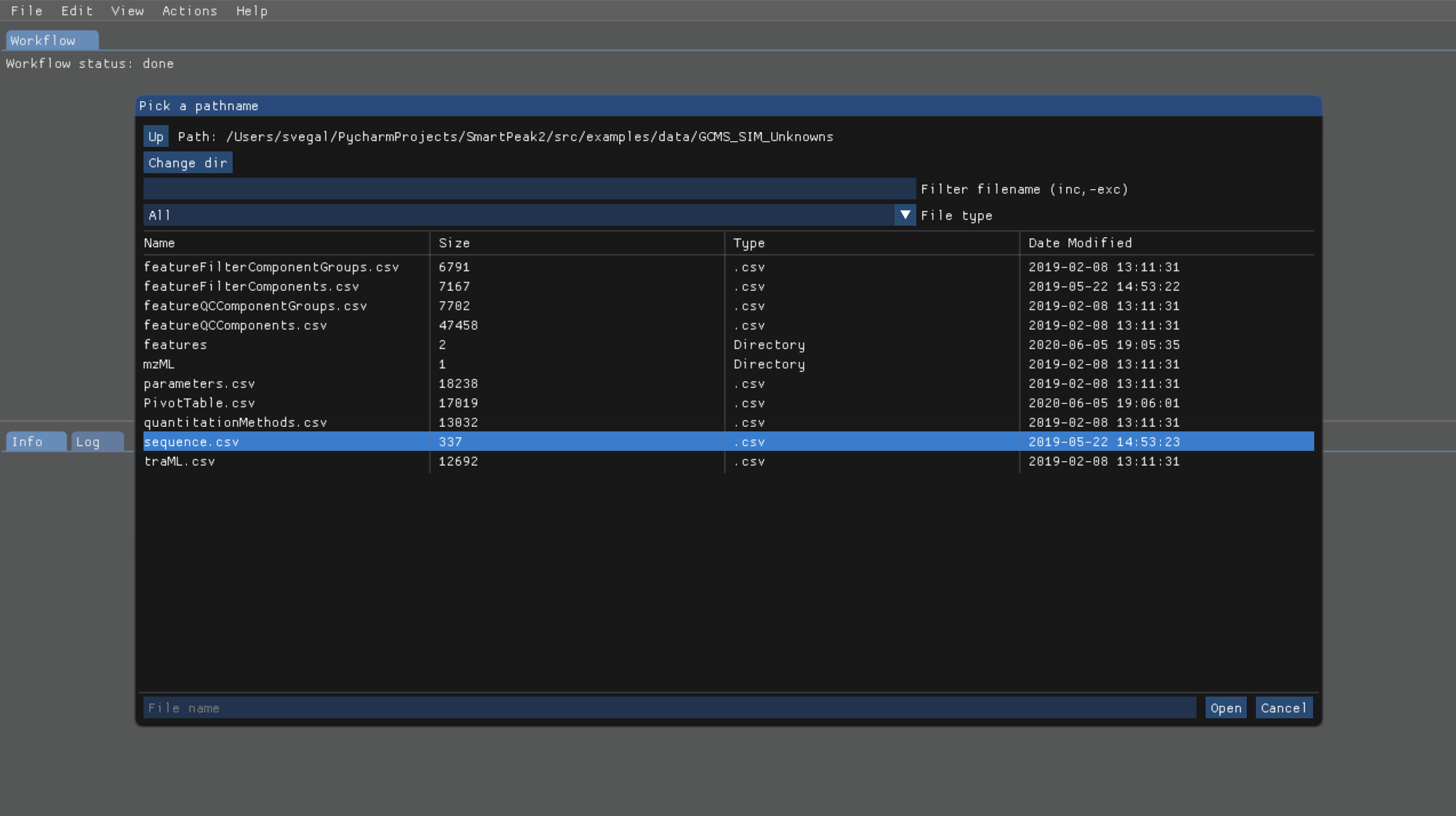
The integrity of the loaded data can be checked with
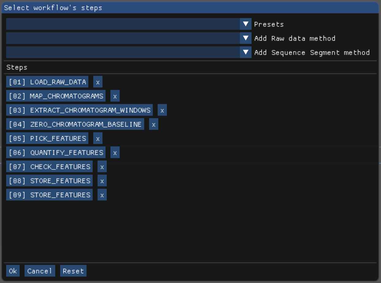
Actions | Integrity checks. The results of the integrity checks can be viewed withView | Info.Edit the workflow with
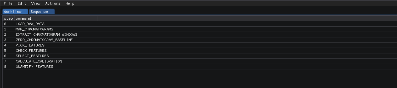
Edit | Workflow. You have an option to cherry pick the custom workflow or to choose the predefined set of operations. For example, the workflow steps for GC-MS SIM Unknowns are the following:
View and verify the workflow steps and input files with
View | [table].
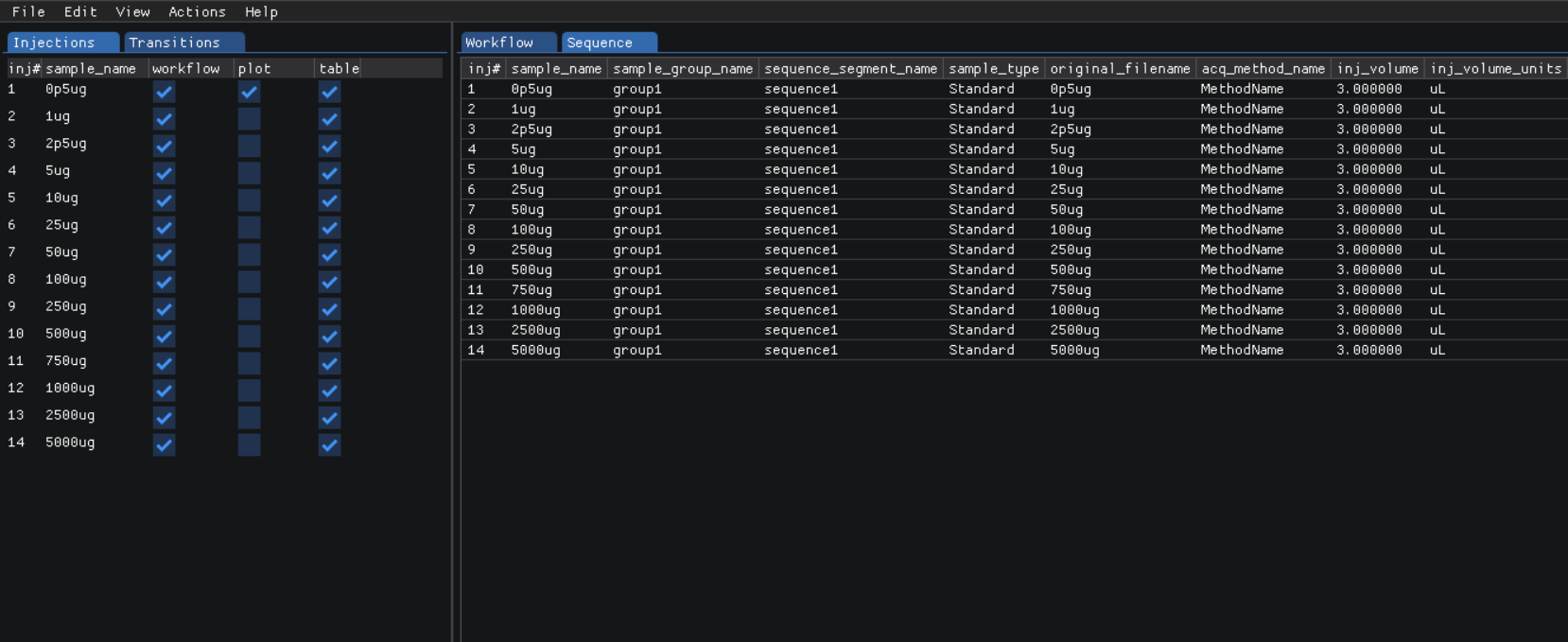
The explorer panes can be used to filter the table views with
View | Injections or Transitions. Click on the checkbox under plot or table to include or exclude the injection or tansition from the view.
Changes to any of the input files can be made by reloading a modified .csv version of the file with
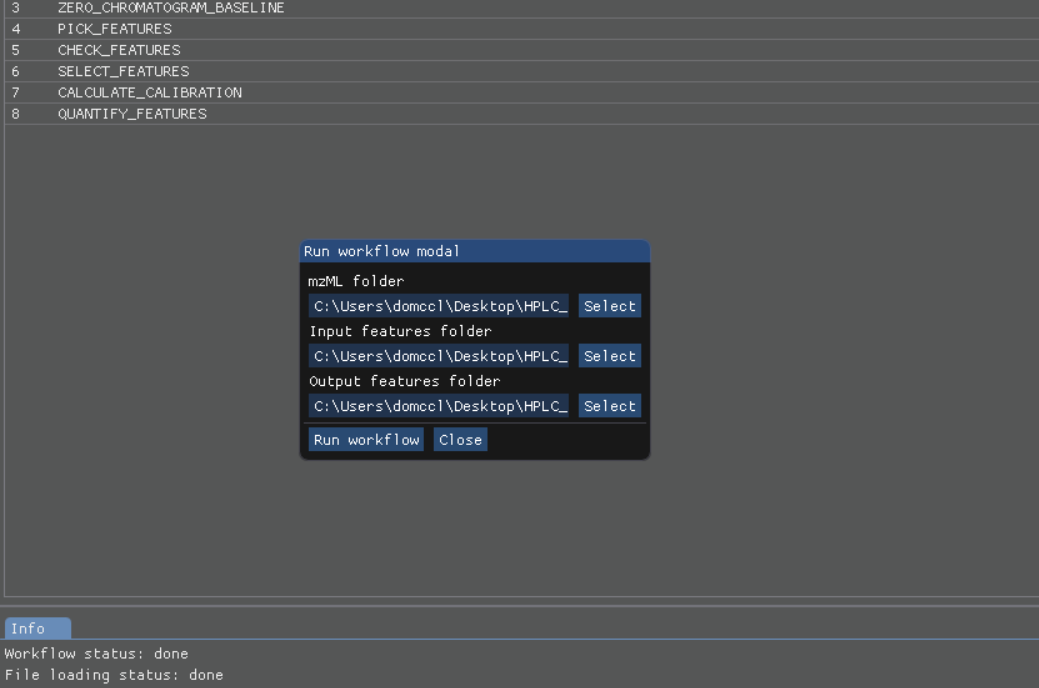
File | Import File.Run the workflow with
Actions | Run workflow. Verify or change the data input/output directories before running the workflow.
The status of the workflow can be monitored with
View | info. An estimated time is available. This value is only a rough estimation. It will be updated regaluary while the workflow is running. The progress bar however shows workflow steps completed. As some steps can be longer to execute, it may not reflect remaining time. More details are available about the items that are currently running.

Alternatively, a more detailed status can be obtained with
View | logwhich will display the most recent SmartPeak log information.

After the workflow has finished, the results can be viewed in a tabular form as a large data table with
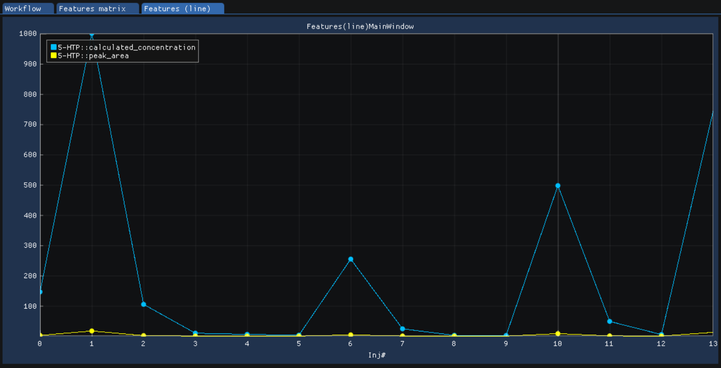
View | features (table). The feature metavalues shown can be added or removed withView | Featuresand clicking on the checkboxes under plot or table. For performance reasons, the amount of data that one can view is limited to 5000 entries.The results can be viewed in a graphical form as a line plot or as a heatmap with
View | features (line).
or View | features (heatmap)

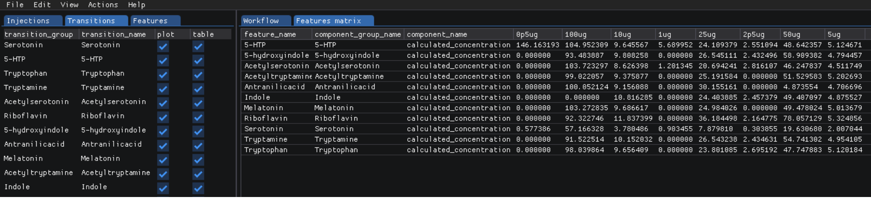
The underlying data can also be displayed as a table matrix with
View | features (matrix). Samples, transitions, or feature metavalues can be included or excluded from any of the views using the explorer panes.
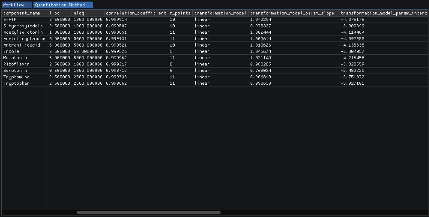
The results of calibration curve fitting can be inspected with
View | Workflow settings | Quant Methods.
A detailed look at the calibration fitted model and selected points for the model can be seen with
View | Calibrators.

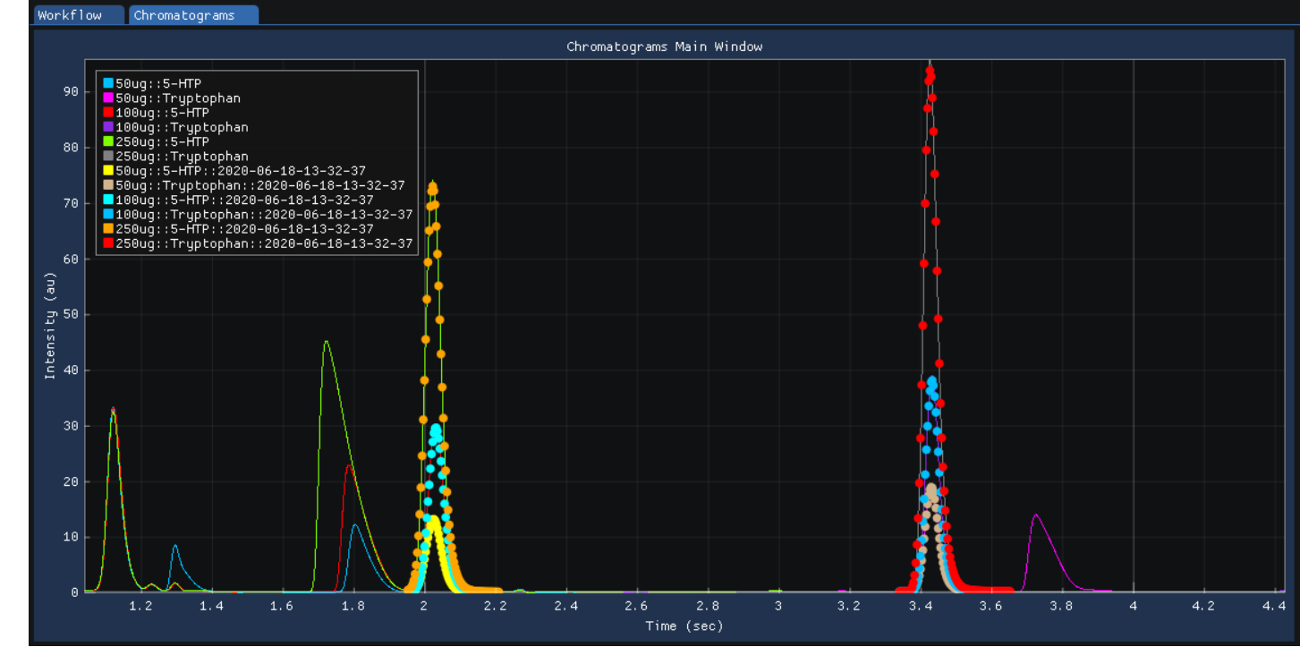
For debugging problematic peaks, the raw chromatographic data and the picked and selected peaks can be viewed graphically with
View | Chromatograms. For performance reasons, the amount of data that one can view is limited to 9000 points.
Export the results with
Actions | Report. There is an option to choose the set of variables of interest
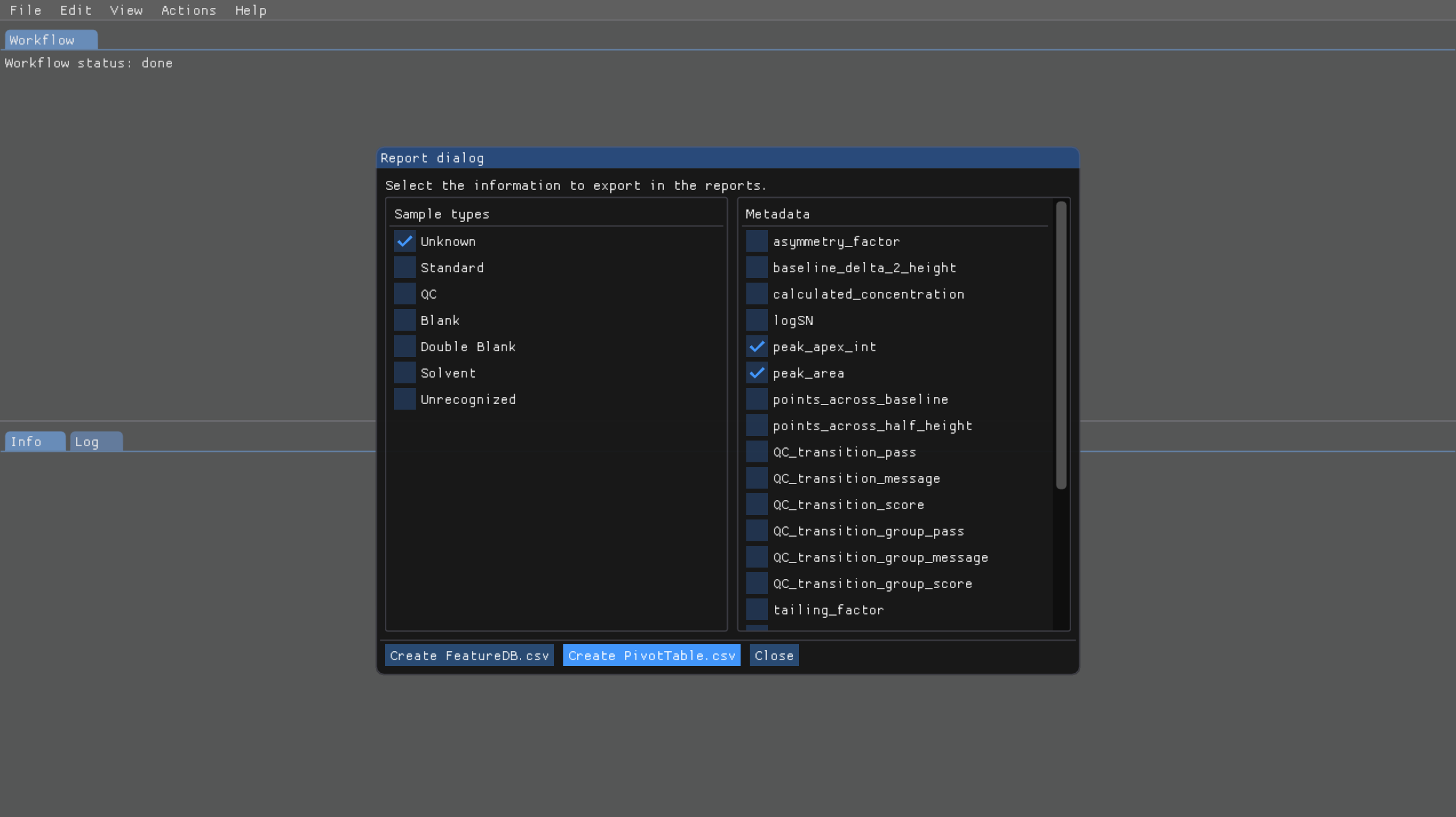
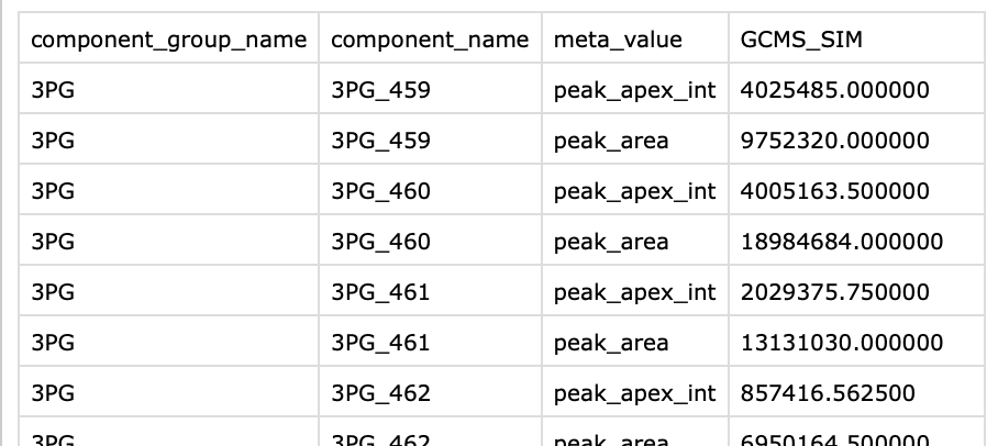
The results will be exported to
PivotTable.csvin the same folder
The above applies for Mac and Linux.