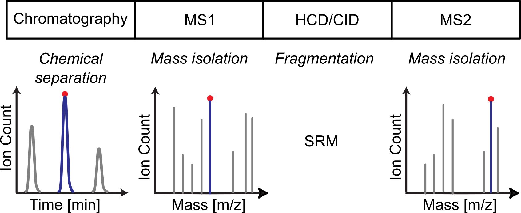
Targeted quantitation using LC-MS/MS-SRM acquisition

This tutorial walks you through the workflow for analyzing targeted single reaction monitoring (SRM) data starting from input file generation, to processing the data in SmartPeak, to reviewing the data in SmartPeak, to reporting the results.

Objectives

1. Obtaining the SOP for the workflow.

2. Choosing a data set for demonstrating the workflow.

3. Creating an optimized SmartPeak input templates for running the workflow.

The Workflows include

1. Calculating the calibration curves to generate quantitation methods for each component using Standard samples

2. Processing Unknown samples using the quantitation methods

Notes

The algorithm parameters used in the following workflows have been highly tuned for feature detection using the Sciex 5500 QTRAP and 6500+ systems with Shimadzu and Agilent HPLC systems. With that said, we have found the algorithm parameters to generalize well to most liquid chromatography coupled to mass spectrometry systems.

Steps

The tutorial includes the following steps :

1. Setting up the input files

The data set used can be found in LCMS_SRM_Standards, LCMS_SRM_QCs, and LCMS_SRM_Unknowns for the LC-MS/MS-SRM Standards, QCs, and Unknowns, respectively.

1. Defining the workflow in SmartPeak

For LC-MS/MS-SRM Standards analysis, the following steps are saved into the workflow.csv file. Alternatively, steps can be replaced, added or deleted direclty from SmartPeakGUI. A detailed explanation of each command step can be found in Workflow Commands.

workflow_LCMSSRM_Standards.csv

workflow_step
LOAD_RAW_DATA
MAP_CHROMATOGRAMS
PICK_MRM_FEATURES
CHECK_FEATURES
SELECT_FEATURES
CALCULATE_CALIBRATION
STORE_QUANTITATION_METHODS
QUANTIFY_FEATURES
STORE_FEATURES

The calibration curve for each transition’s quantitation method can be inspected after all workflow steps have been run, to do so please click on view and then “Calibrators”. From the menu select ser-L.ser-L_1.Light as component to plot its concentration curves within the given concentration range as shown below:

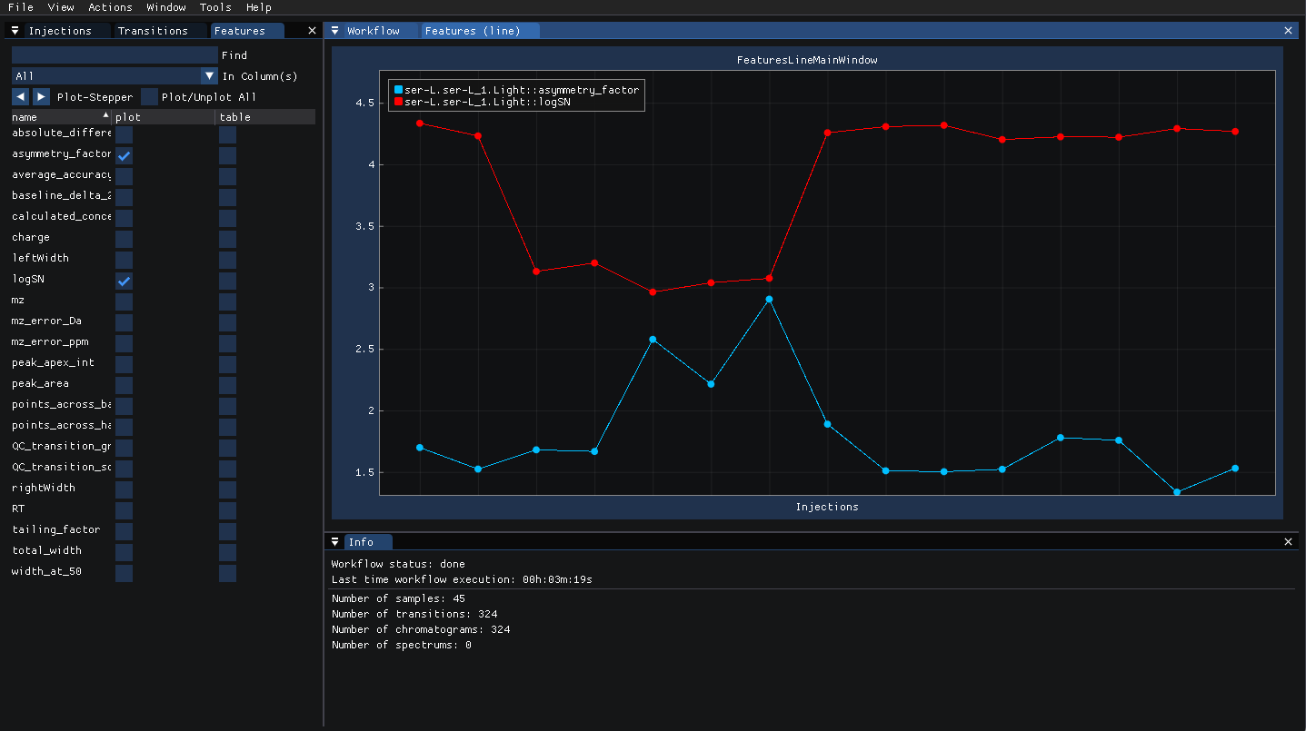
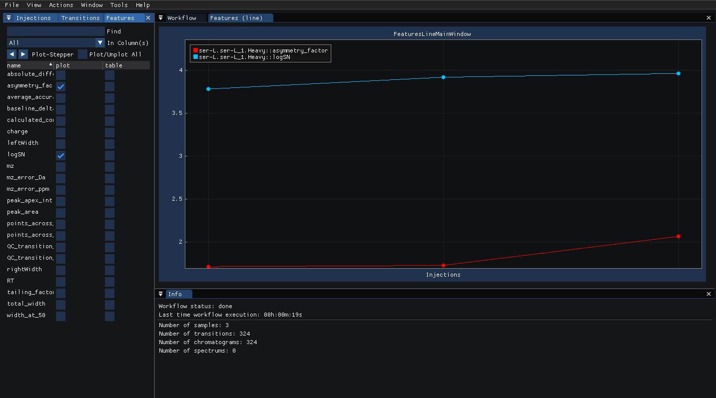
To inspect the features for the selected transition groups, select “Features (line)” from the view menu then open the features tab (can be opened from the view menu as well) to select the “asymetry_factors” and “logSN” in the plot column. The line plot illistrates the value for each transition group and feature as shown below:

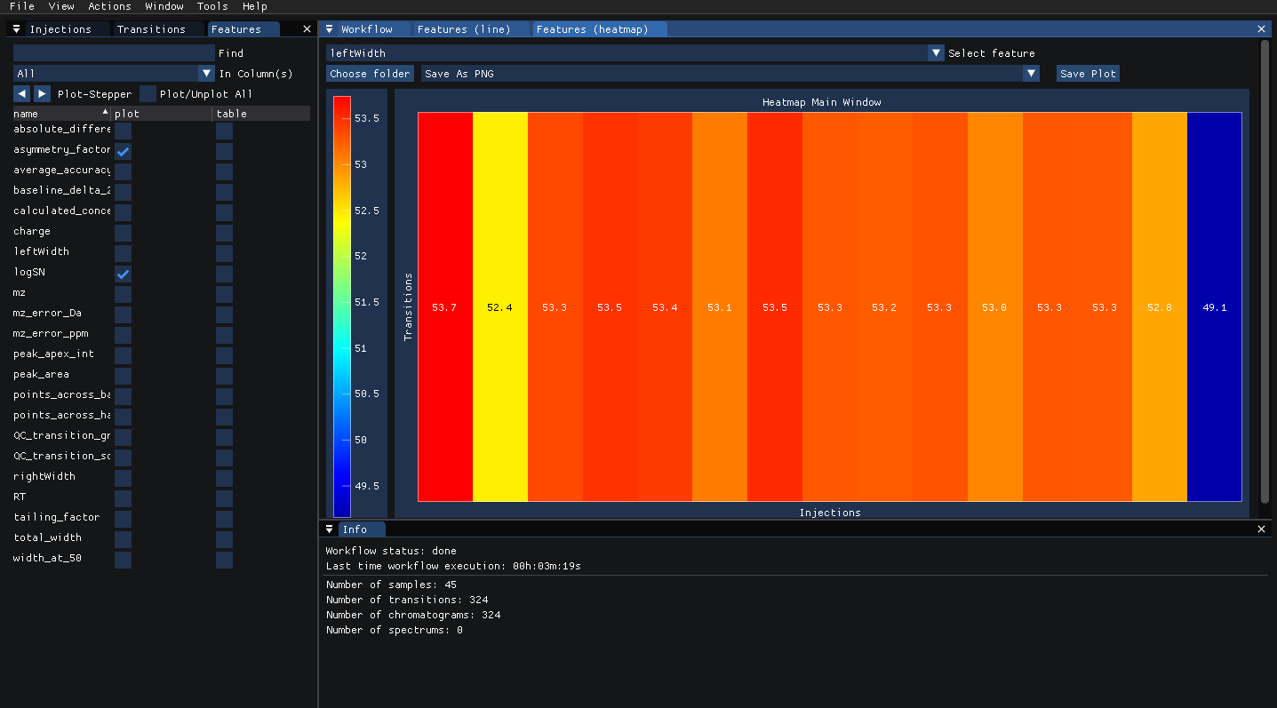
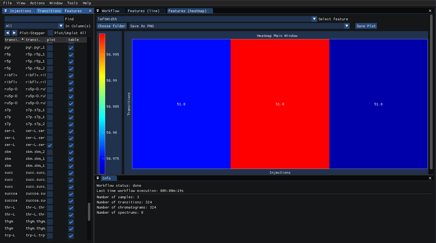
The features can also be plotted as a heatmap, under “view” select “Features (heatmap)” then select the “left_width” feature to display transition groups as a heatmap and compare the values from the same injection as shown below:

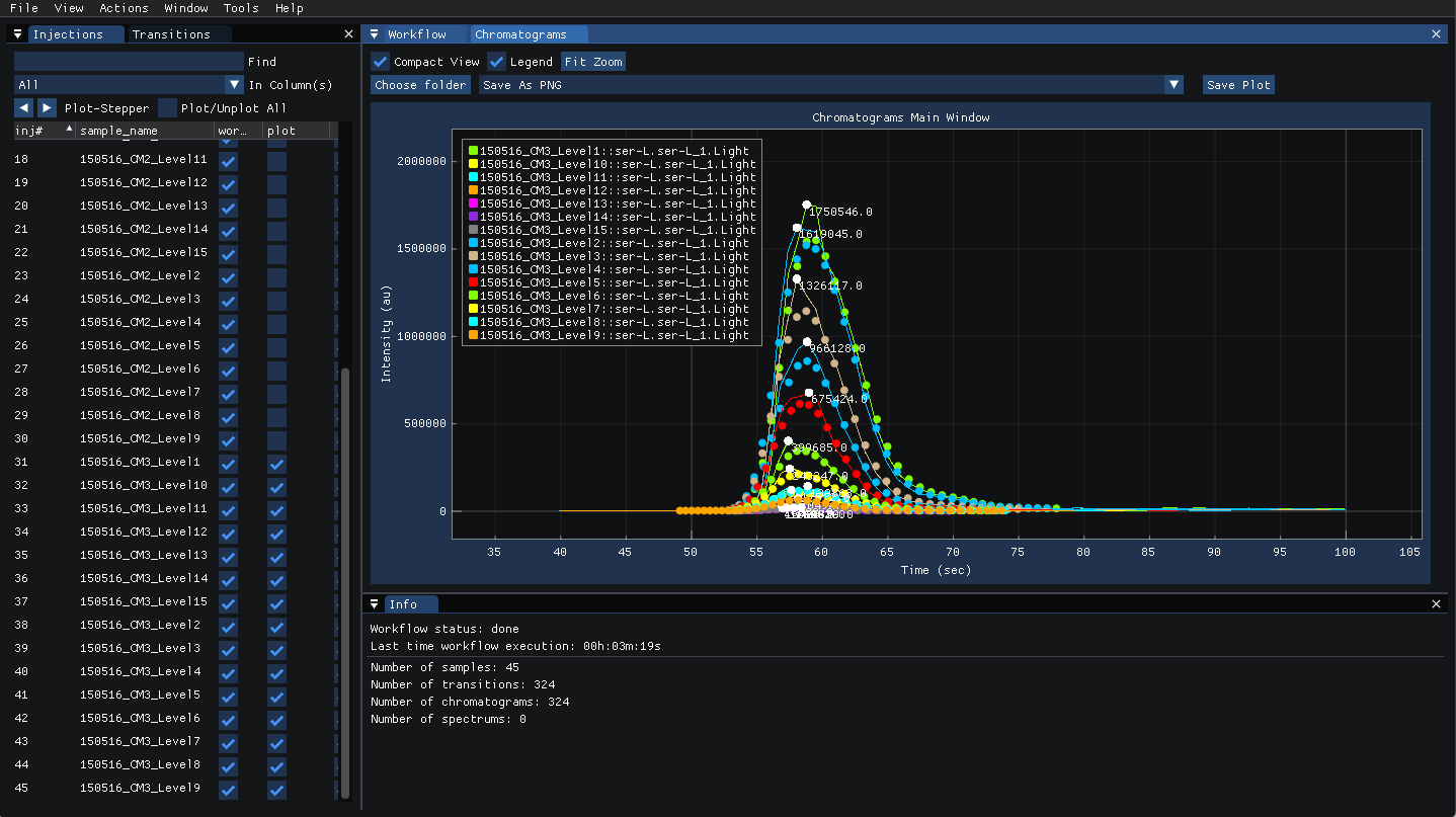
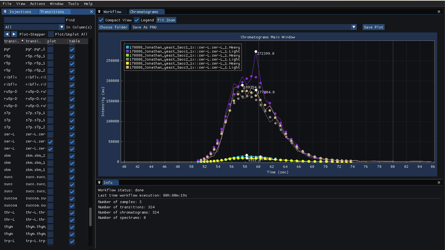
To plot the intensities over time for given injections and transitions, view the “chromatogram” from the “view” menu then select the injections and transitions to plot from their respective tabs on the left. The following shows the chromatograms for the calibration mix 3 (CM3) series of Standards for L-serine light and heavy transitions.

The workflow step STORE_QUANTITATION_METHODS writes the calibration model for each transition, an excerpt can be seen below:

Generated sequence1_quantitationMethods.csv

IS_name	component_name	feature_name	concentration_units	llod	ulod	lloq	uloq	correlation_coefficient	n_points	transformation_model	transformation_model_param_y_weight	transformation_model_param_y_datum_min	transformation_model_param_y_datum_max	transformation_model_param_x_weight	transformation_model_param_x_datum_min	transformation_model_param_x_datum_max	transformation_model_param_symmetric_regression	transformation_model_param_slope	transformation_model_param_intercept
23dpg.23dpg_1.Heavy	23dpg.23dpg_1.Light	peak_apex_int	ug/mL	0.0	0.0	0.0025	50.0	0.998429475730303	4	linear	ln(y)	-1.0e15	1.0e15	ln(x)	-1.0e15	1.0e15	FALSE	0.36817238220267	2.65567855569643
23dpg.23dpg_1.Heavy	23dpg.23dpg_2.Light	peak_apex_int	ug/mL	0.0	0.0	1.0	50.0	0.996468124200467	4	linear	ln(y)	-1.0e15	1.0e15	ln(x)	-1.0e15	1.0e15	FALSE	1.14095656824418	-0.440569296738733

This file is used to apply the predefined calibration model to each transition by running the QUANTIFY_FEATURES workflow step.

The workflow steps for LC-MS/MS-SRM Unknowns are :

workflow_LCMSSRM_Unknowns.csv

workflow_step
LOAD_RAW_DATA
MAP_CHROMATOGRAMS
PICK_MRM_FEATURES
QUANTIFY_FEATURES
CHECK_FEATURES
SELECT_FEATURES
STORE_FEATURES

To inspect the features for the selected transition groups, select “Features (line)” from the view menu then open the features tab (can be opened from the view menu as well) to select the “asymetry_factors” and “logSN” in the plot column. The line plot illistrates the value for each transition group and feature as shown below:

The features can also be plotted as a heatmap, under “view” select “Features (heatmap)” then select the “asymetry_factors” feature to display transition groups as a heatmap and compare the values from the same injection as shown below:

To plot the intensities over time for given injections and transitions, view the “chromatogram” from the “view” menu then select the injections and transitions to plot from their respective tabs on the left. The following shows the chromatogram for three injections for L-serine light and heavy transitions.

1. Running the workflow in SmartPeak

   To run the analysis, please follow the steps for Using SmartPeak GUI or Using SmartPeak CLI to execute the workflow steps, review the results, and report the results.

2. Reporting the results

   To export the results, select “Report” from the “Actions” which will show the “Create Report” window:

   

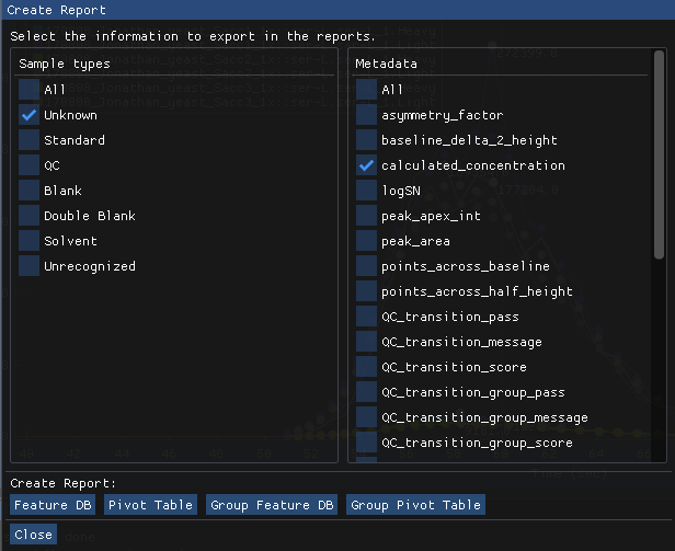
   Based in the data you wish to export, select the desired “Sample types” from the left pane and select the “Metadata” from the right pane then click on of the buttons below to create the report with the selected items in the csv format. More details on exporting the results can be found in Export report.